Lab 10: Object-based Classification

Background and Goal

In this lab, we learn how to utilize object-based classification in eCognition. This method of classification is state-of-the-art, and uses both spectral and spatial information to classify the land surface features of an image. The first of three steps in this process is to segment an image into different homogenous clusters (referred to as objects). This is then followed by selecting training samples to be used in a nearest neighbor classifier, an algorithm which is then used with the samples to create a classification output.

Methods

As stated previously, the first step in object-based classification is to segment the image into different objects. This is done by incorporating a false color infrared image into a multiresolution segmentation algorithm within eCognition’s ‘Process Tree’ function. For this classification, a scale parameter of 10 was used. This determines how detailed or broad the segments are. After this process is executed, it categorizes the different features in the image, splitting them as different objects. Figure 1 shows the different objects that were generated for the Eau Claire area.

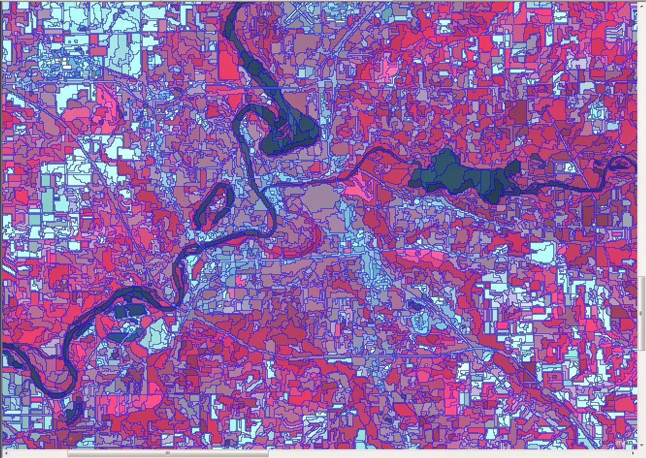
Figure 1: An example of the segmentation that was created to differentiate between the different 'objects' of the image.

It is then necessary to create classes for the object-based classification. In the ‘Class Hierarchy’ window of eCognition, five different classes were inserted. The classes we used were Forest, Agriculture, Urban/built-up, Water, and Green vegetation/shrub. Each of these classes was assigned a different color. After this, the nearest neighbor classifier was applied to the classes, with the mean pixel value selected for the objects’ layer value. This will be the classifying algorithm for the process. Once this is complete, samples are selected in a much similar way to supervised classifications. Four objects in each class were selected and used as samples for the nearest neighbor classification. A new process was then created in the process tree, and the classification algorithm was assigned. Once this process was executed, the image becomes classified. It was then necessary to manually edit the image to change objects that had been falsely classified. The results were then able to be exported as an ERDAS Imagine Image file, to be further analyzed in a more familiar program.

Results

Figure 2 shows the result of the classification. This classification process was fairly simple to use, and produced beautiful results. Urban/built-up is still slightly under predicted, but overall the image looks quite accurate.

Figure 2: The final result of the object-based classification technique.

Sources

Earth Resources Observation and Science Center. (2000). [Landsat image of the Eau Claire and Chippewa Counties]. United States Geological Survey. Obtained from http://glovis.usgs.gov/

Lab 9: Advanced Classifiers II

Background and Goal

In this lab, we learn about two more advanced classification algorithms. These algorithms produce classification maps that are much more accurate than those that are created with simple unsupervised and supervised classifiers. Specifically, this lab explores the use of an expert system classification (using ancillary data), and the development of an artificial neural network (ANN) classification. Both of these functions use very robust algorithms to create complex and highly accurate classification maps.

Methods

The use of expert systems is applied to increase the accuracy of previously classified images using ancillary data. In this lab, we used a classified image the Eau Claire, Altoona, and Chippewa Falls area (Figure 1). The map had the classes of Water, Forest, Agriculture, Urban/built up, and Green vegetation. In this classification map, Agriculture and Green Vegetation classes were over predicted. To use the expert system to correct these errors, it is first necessary to construct a knowledge base. Knowledge bases are built up of hypotheses, rules, and variables. Hypotheses are the targeted LULC classes, rules are the functions that will be used to classify the hypotheses, and variables are the inputs (previously classified image and ancillary data). For this lab, we created eight hypotheses. One was for water, one was for forest, one was for residential, one was for other urban, two were for green vegetation, and two were for agriculture. There are more hypotheses than classes because there must be a hypothesis for each correction. In the exercise, we broke the urban/built up class into ‘Residential’ and ‘Other Urban’, corrected green vegetation areas that were predicted as agriculture, and corrected agriculture areas that were predicted as green vegetation. The functions used bitwise language to classify the different hypotheses using the previously classified image and the ancillary data. Figure 2 shows the complete knowledge base. Once the knowledge base was complete, the classification was run producing a classification image with the eight hypotheses. These were then recoded into the six classes (basically just merging Green Vegetation with Green Vegetation 2 and merging Agriculture with Agriculture 2) complete the classification.

Figure 1: The original classified image of the Eau Claire, Altoona, and Chippewa Falls area.

Figure 2: The complete knowledge base. The hypotheses are on the left (green boxes), with corresponding rules on the right (blue boxes). There is a counter argument for each classifying argument.

ANN simulates the process of the human brain to perform image classification by ‘learning’ the patterns between remotely sensed images and ancillary data. It uses input nodes, hidden layers, and output nodes to bounce information back and forth and reveal the best answer based on the different Training Rates, Training Momentums, and Training Thresholds. In this lab, we used high resolution imagery of the University of North Iowa. To conduct the ANN classification, it was first necessary to create a training sample, by highlighting Regions of Interest (ROI). These ROI’s are essentially the classes that the image will be classified into. For this classification, the ROI’s were Rooftops, Pavement, and Grass. Figure 3 shows the reflective image with ROI’s highlighted. These ROI’s were then used as ancillary data in the ANN classification, with a Threshold of 0.95, a Training Rate of 0.18, and a Training Momentum of 0.7.

Figure 3: The image of UNI's campus overlayed with ROI's of grass (green), rooftop (red), and pavement (blue).

Results

The expert system classification produced a much more accurate image than the previous classified image. The image corrected the over prediction of agriculture and green vegetation, as well as creating two classes for the urban/built up class. Figure 4 shows the result of the expert system classification.

Figure 4: The result of the expert system classification method. It is much more accurate than the previous image.

The ANN classification was surprisingly easy to use, and produced an easily readable classification image. Figure 5 shows the results. It is easy to tell where the roads and the grass are. However, it classified the trees as rooftops (due to their shadows), and some of the rooftops were classified as pavement. Though the image isn't terribly accurate, it is surprisingly easy to distinguish between features, considering the work that the analyst has to do.

Figure 5: The classification image of the ANN classification method. Green areas are grass, blue areas are pavement, and red areas are rooftops.

Sources

Earth Resources Observation and Science Center. (2000). [Landsat image of the Eau Claire and Chippewa Counties]. United States Geological Survey. Provided by Cyril Wilson.

Department of Geography. (2003). [Quickbird High Resolution image of the University of Northern Iowa campus]. University of Northern Iowa. Provided by Cyril Wilson.

Lab 8: Advanced Classifiers I

Background and Goal

The goal of this lab is to learn two advanced classification algorithms. These advanced classifiers are much more robust, and produce a classified image that is more accurate than those produced by unsupervised and supervised classifiers that were used in previous labs. The two algorithms that are learned in this lab are Spectral Linear Unmixing and Fuzzy classification. Spectral Linear Unmixing utilizes the measurement of ‘pure’ pixels (also known as endmembers) to classify images. Fuzzy classification accounts for mixed pixels in an image. Some pixels are a combination of several classes (due to spectral resolution) and thus membership grades are used to determine which class is more strongly identified within the pixel.

Methods

To conduct a spectral linear unmixing classification, it was first necessary to transform the image into a Principal Components (PC) image. This technique compiles all information into more compact bands, providing most of the image’s information within the first two to three bands in the PC image. This function was done with ENVI. For our image, most of the information was compiled in bands 1 and 2 of the PC image, with some information in band 3. To collect endmembers from the PC image, we created scatterplots of the informational bands. First, a scatterplot was generated with band 1 and the x-axis and band 2 and the y-axis. This created a scatterplot with a triangular shape. The points of this triangle are the ‘pure’ pixels (endmembers). These points were selected and turned into a class. The first scatter plot included the endmembers for water, agriculture, and bare soil (Figure 1 shows this scatterplot). However, to complete the classification, we also need endmembers for the urban class. We created a second scatterplot of bands 3 and 4 to collect these endemembers (Figure 1 shows this scatterplot as well). The endmembers are also highlighted on the reference image to make sure that the correct endmembers were selected (Figure 2). All of these endmembers were then exported into a region of interest (ROI) file and were then used in the Linear Spectral Unmixing function in ENVI, producing fractional maps for each endmember.

Figure 1: The scatterplots used to collect endmembers. The colors correspond to the colors in the reference map in Figure 2.

Figure 2: The reference map for collecting endmembers. The areas highlighted with green are the bare soil endmembers, yellow are the agriculture endmembers, blue are the water endmembers, and purple are the urban endmembers.

The processing for fuzzy classification was all executed within ERDAS. The first step is to select signatures from the input image. These signatures must be from areas where there is a mixture of land cover classes, as well as homogenous land cover. The aoi’s for the signature samples had to contain between 150 and 300 pixels. Four samples were collected for the water, forest, and bare soil classes, and six samples were collected for the agriculture and urban/built up classes. The samples for each of the classes were then merged, to create one aggregated sample for each class. These signatures were then used to create a fuzzy classification with ERDAS’ supervised classification function. This first function creates five layers of classified images, ranking the most probable classes for each pixel. A fuzzy convolution algorithm was then used in ERDAS to turn these layers into one classified image.

Results

Figures 3 through 6 show the results of the linear spectral unmixing function. The bare soil fractional map is quite accurate. It highlights the bare area surrounding the airport very well, as well as the empty crop fields to the east and the west. The fractional map for agriculture is a little less accurate. It seems to slightly highlight vegetation in general, and not just agriculture areas. The water fractional map is surprisingly inconsistent. Usually water is easy to classify, and it was classified well. However, the map also classified areas that were not water (notably the area around the airport). The urban fractional map worked surprisingly well. It successfully highlights the urban areas, but fails to leave other areas in the dark.

Figure 3: The Bare Soil fractional map.

Figure 4: The Agriculture fractional map.

Figure 5: The Water fractional map.

Figure 6: The Urban fractional map.

Figure 7 shows the final result of the fuzzy classification. This classification worked much better than the supervised classification in the previous lab, though the urban and agriculture classes were still over predicted.

Figure 7: The final result of the fuzzy classification.

Sources

Earth Resources Observation and Science Center. (2000). [Landsat image of the Eau Claire and Chippewa Counties]. United States Geological Survey. Provided by Cyril Wilson.