Lab 11: Lidar Remote Sensing

Background and Goal

Lidar is a rapidly expanding field in the remote sensing world. It has shown significant growth in recent years, due to its impressive and high tech nature. The main goal of this lab is to experience Lidar processing, as well as gaining knowledge of Lidar data structure. Specifically, we learn how to process and retrieve the different surface and terrain models and how to create derivative images from the point cloud. These images show first return hillshading (which gives a 3D looking, imitation aerial image), ground return hillshading (which reveals the elevation of the landscape itself), as well as intensity imagery (which shows a high contrast grayscale image, much like those of the Landsat panchromatic band).

Methods

The first step in Lidar processing is to create a LAS as Point Cloud file, and add the different LAS tiles within the study area. This was done within ArcMap, by creating a LAS dataset and adding the LAS files to the dataset. Because Lidar data is so big, the study area is composed of several LAS tiles. These files were then examined to determine if they are resembling the area of interest. This was done by looking at the Z values (or elevation) of the points. Since the minimum and maximum Z values matched the profile of Eau Claire, the data was determined to be useful. The dataset was then projected into the correct XY and Z coordinate systems by examining the metadata. Our data used the NAD 1983 HARN Wisconsin CRS Eau Claire projection for the XY coordinates, using feet as the unit. The NAVD 1988 projection was used for the Z coordinates, with feet as the unit as well. We then used a previously projected shapefile of the Eau Claire County to make sure that the dataset was properly projected.

Using the LAS Dataset Tool, we were then able to apply different filters to the dataset in order to further analyze the Lidar points. It was possible to examine the different classes that were assigned to each point (Ground, Building, Water, etc.), as well as elevation differences, slope ratios, and contour lines.

In order to create a Digital Surface Model (DSM), we used a LAS dataset to Raster conversion tool. It was necessary to adjust the sampling value so that it did not exceed the nominal pulse spacing. If the sampling value were finer than the nominal pulse spacing, the data would be inaccurate. This model used First Return points (points that are immediately reflected), to reveal the topmost surfaces of objects in the study area. This process created a black and white raster image, which was then converted into a hillshade image to give a 3D effect.

The production of a Digital Terrain Model (DTM) was executed in a much similar manner. This time, a filter was applied to use the Lidar points that were classified as Ground. This effectively removes buildings and vegetation from the DSM, leaving only the open earth. The process created a black and white raster image, which was then converted to a hillshade image to give a 3D effect. DTMs are very beneficial because they easily reveal the elevation patterns of the study area.

Lastly, an Intensity image was created. This image reveals the intensity of returns of the Lidar data. Areas with higher frequencies show up lighter on the image, while areas with lower frequencies show up darker on the image. This image was created using the same process as both the DSM and the DTM, but instead of measuring elevation, the process measured point intensity.

Results

Figure 1 shows the hillshade DSM image, Figure 2 shows the hillshade DTM image, and Figure 3 shows the Intensity image. Note the effects that water has on the images in all three figures. In the DSM and DTM, the water looks strange because of the lack of point density in those areas.

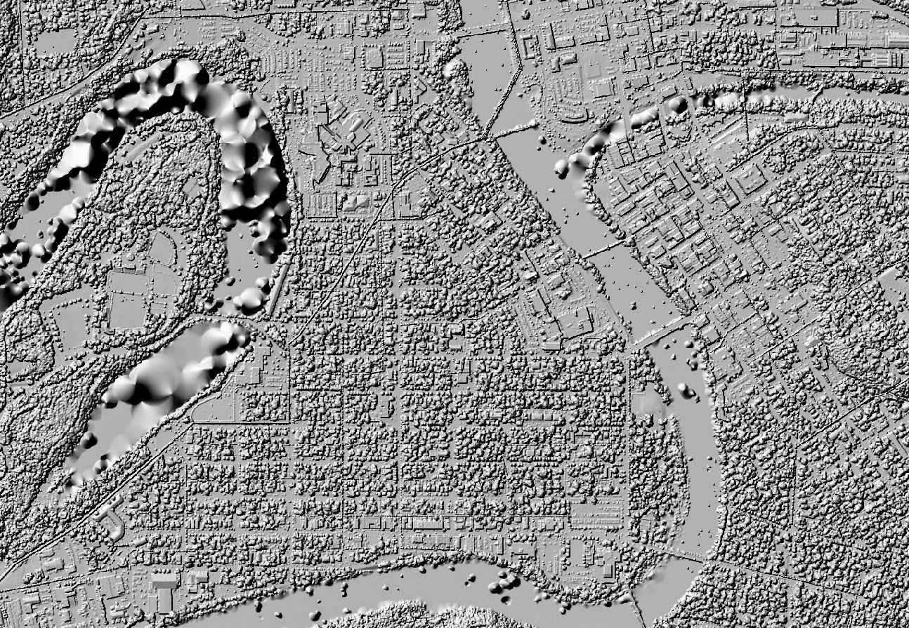Figure 1: The DSM image. This image was created using first return points, so it is as if we are actually viewing the landscape from above.

Figure 2: The DTM image with hillshading applied. This image highlights the raw elevation differences throughout the study area, with little obstruction from vegetation and buildings.

Figure 3: The Intensity image. Urban surfaces are lighter because more pulses were reflected and thus returned. Vegetation and water are darker because more pulses were absorbed, so fewer returned.

Sources

Eau Claire County. (2013). [Lidar point cloud data]. Eau Claire County. Obtained from Eau Claire County.